#

# Compounding, Expected Returns, and Volatility

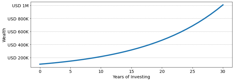
Compounding is one of the miracles of investing. If you invest USD 100K and your portfolio returns 8% every year after 10 years, you'll have USD 216K, after 20 years, USD 466K, and after 30 years, a cool USD 1M. It grow exponentially. Practically the reason for this is that in the second year, you earn interest on your interest. In the third year, you earn interest on the interest on your interests, and so on...

Variation in returns turns out to be your enemy. Imagine that you invest USD 1 for two years. The first year you gain 10%, and the second year you lose 10%. Your average return is 0, but how much money do you have at the end? For any return r

(1 + r) \times (1-r) = 1 +r - r -r^{2} = 1 - r^2

If r=10\%, at the end of two years, instead of a dollar, you only have 99 cents. This doesn't look like much, but over time variation in returns makes a portfolio compound a lot slower.

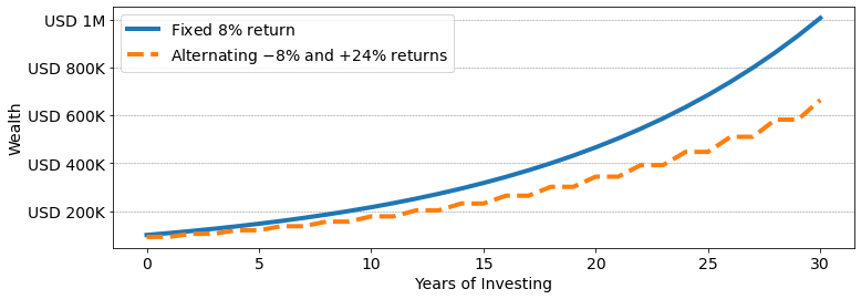
Imagine that your portfolio alternates good and bad years. In bad years you lose 8\%, and in good years, you gain 24\%. Your average return is still 8\% = (-8\% + 24\%) / 2. But your portfolio compounds much more slowly. At the end of 30 years, you'll have USD 663K instead of USD 1M.

The variation of returns around their mean is called the volatility of the returns. Formally, if you have a sequence of returns r_1, r_2, \cdots, r_n, with mean \overline r = \frac{1}{n}(r_1 + r_2 + \cdots r_n) the volatility of those returns is

\text{v} = \sqrt{\frac{1}{n} \sum_{k=1}^n (r_k -\overline r)^2}

When you look at returns over short time intervals (say daily returns) so that returns are small, a portfolio with returns r_1, r_2,\cdots, r_n, compounds approximately at the same speed as a portfolio with fixed return equal to

\underline r = \overline r- v^2/2.

Volatility makes portfolios compound slower.

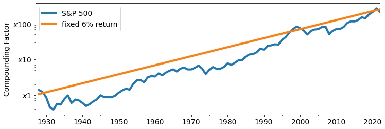
For instance, over the last 90 years, the yearly returns of the S&P 500 are approximately 8%, with a yearly volatility of about 20%. This means that a portfolio invested into the S&P 500 will compound like a portfolio with a fixed return of 6%:

6\% = 8\% - 20\% \times 20\% / 2.

# The diversification free lunch and regular rebalancing

Take two assets A and B. Asset A has returns r_1^A, r_2^A, \cdots, r_n^A, while asset B has returns r_1^B, r_2^B,\cdots, r_n^B. Imagine that both assets have the same expected yearly returns and volatility as the S&P 500: an 8% return, and 20% volatility.

As we've just seen, each asset compounds roughly at a 6% rate.

Now imagine that you diversify. You follow a regular rebalancing strategy in which each January 1st, you rebalance your assets so that 50% of your wealth is in asset A, and 50% of your wealth is in asset B. This means that each year your portfolio will have returns

r^{50/50}_1 = \frac{1}{2} r^A_1 + \frac{1}{2}r^B_1\quad,\quad r_2 = \frac{1}{2} r^A_2 + \frac{1}{2}r^B_2\quad,\quad \cdots \quad, \quad r_n = \frac{1}{2} r^A_n + \frac{1}{2}r^B_n.

This means that the 50/50 portfolio also has an average return of 8%. The beauty of diversification is that the volatility of the 50/50 portfolio is not 20%. Frequently, the negative shocks experienced by one asset will be compensated by the shocks to an other asset. In particular, if the two assets have independent returns, then the 50/50 portfolio has a variance 20\% / \sqrt{2} \simeq 14\%!

This means that the 50/50 portfolio will compound faster than each of the underlying assets.

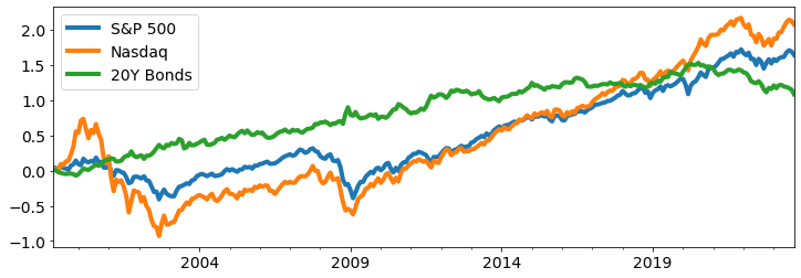
An example. Consider a regular rebalancing strategy assigning 50% weights to the S&P 500 and to 20 Year US Treasury Bonds. Over the 50 years from 1970 to 2020, the S&P 500 and 20Y Bonds have similar yearly returns and volatility: roughly 9% returns and 17% volatility, although 20Y Bonds end up performing better. Over 50 years, the S&P500 multiplies wealth by 40, and 20Y Bonds by 50. A 50/50 Rebalancing strategy multiplies wealth by 60.

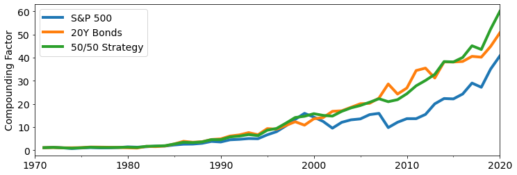
A really surpising fact is that even though the S&P500 performs less well than 20Y Bonds over this period, combining the two together yields an asset that performs better than both.

Note that this would not happen if you invested 50% of your wealth in each asset in 1970 and never rebalanced. In that case your compounding factor would be the average of the compounding factors for the S&P 500 and 20Y Bonds: a factor of 45. Regular rebalancing is needed for your portfolio to outperform each of the underlying assets.

The reason for this is that if you don't rebalance, then over time your allocation will fluctuate away from 50/50 weights, reducing your diversification. For instance, starting from 50/50, after an equity bull run, you may end up with a 70/30 allocation. Inversely, after an equity crash, you may end up with a 30/70 allocation. This leaves you poorly positioned to deal with the next market scenario.

An important caveat. Allocating your portfolio to multiple assets only reduces volatility if the assets don't move the same way. If the assets always move in the same direction they do not diversify each other very well. Correlation is a measure of how well two assets diversify one another. It takes values between 1 and -1. When correlation is 1, the shocks to the two assets are always in the same direction. When correlation is -1, the shocks to the two assets always compensate one another.

For instance the S&P 500's correlation with the Nasdaq is 90% while its correlation with 20Y Bonds is -30%. This means that on average, 20Y Bonds have offered better diversification benefits than Nasdaq to equity holders.

# Drawdowns

We now come to drawdowns, or more precisely (and this will matter later) drawdowns vs the safe asset. The drawdown of a portfolio against a safe asset like cash, is loss in value between the historical peak of the portfolio, and the current value. Formally, the drawdown at time t is

\text{Drawdown}_t = 1- (\text{Porftolio Value}_t / \text{Peak Historical Value}_t)

The maximum drawdown of a portfolio over a time period correspond to the biggest Peak-to-Trough loss experienced by the portfolio. The maximum drawdown for the Nasdaq index is quite remarkable. From March 2000 to September 2002, the Nasdaq lost 81% of its value.

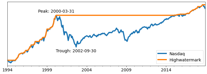
Think about it. This is a remarkable number. If you had invested USD 1000 at the peak, two and a half years later, you'd be left with USD 200.

This is not something that an investor can ignore, even if you are hoping to stay invested for the long run. First, it's an incredible amount of stress to deal with. Instead of riding the storm out, most people who plan to buy-and-hold end up getting cold feet and sell somewhere close to the trough. Second, such drawdowns are really problematic if you need liquidity. Imagine you need to deal with a large expense somewhere close to the trough...

For quantitative asset managers, drawdowns are a key metric, in part because they know that whenever they have large drawdowns, their investors will pull their funds (or at least what's left of them).

We will discuss strategies to minimize drawdowns in the next chapters. For now we want to emphasize 2 facts:

1. Drawdowns and volatility are different and need not be related.
2. Given observed volatility, very large drawdowns, like the one experienced by Nasdaq in the 2000's, should be very rare in an efficient market. The fact large drawdowns they happen tells us something about the dynamics of fear in real markets.

# Drawdowns are not volatility

One way to see that drawdowns are not related to volatility is the reshuffle (i.e. reorder in a random way) the monthly returns of the Nasdaq. Mechanically the reshuffled returns have the same mean return and the same volatility as the Nasdaq. Your total wealth would be the same if you invested in the Nasdaq, or its reshuffled version.

A typical such reshuffling is illustrated below. In the 25 years from 1994 to 2019, both the actual Nasdaq and the Reshuffled Nasdaq have a mean yearly return of 11.5% and a volatility of 25%. However, they have very different drawdowns. While the Nasdaq experiences Peak-to-Trough losses of 81%, the Reshuffled Nasdaq only experiences a Peak-to-Trough loss of 38%. The reason for this is that the reshuffling breaks down persistent patterns in actual Nasdaq returns.

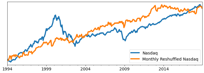
Takeaway: Large Drawdowns in real markets are not the result of volatility, but rather, of a persistent downward trend.

# Drawdowns make a difference to investors

It should be clear to most investors that investing in the Reshuffled Nasdaq is a lot less stressful than investing in the actual Nasdaq, even though they start and end at the same point.

What's less obvious is that if you draw on your savings for consumption, then large drawdowns can reduce your long run wealth. For instance, imagine that in 1994 you invested USD 150,000 in the Nasdaq. Starting in 1994, every month, you sell some of your assets to fund USD 1000 of expenses, rowing at 5% a year. If you invested in the actual Nasdaq, then in 2019, your wealth would be USD 258,000. If you invested in the Reshuffled Nasdaq, your wealth in 2019 would be USD 411,000.

The reason for this is that after a large drawdown, your expenses constitute a larger part of your savings. This reduces the basis on which you compound going forward, potentially resulting in significantly lower wealth.

# Large Drawdowns are Very Rare in an Efficient Market

The contrast between the actual Nasdaq and the Reshuffled Nasdaq is not due to the fact that we picked a very specific reshuffling. The figure below illustrates the distribution of Peak-to-Trough drawdowns obtained from 10,000 independent reshufflings of the Nasdaq. In 99.8% of simulations, the maximum drawdown of the reshuffled Nasdaq is less than the maximum drawdown of the real Nasdaq. In an efficient market where patterns of returns are not predictable, actual drawdowns should not be so far to the right in the distribution of reshuffled drawdowns.

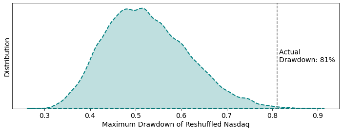
One possible interpretation of this fact is that large drawdowns reflect a market's failure to equilibrate as fear of downturn builds up, resulting in a slow moving crash.

# Performance metrics

Risk-management is at the heart of our work.

Whenever we building portfolios, we monitor the key quantities we have been talking about:

• the yearly return
• the yearly volatility
• maximum and current drawdowns

In addition, it's often helpful to keep track of ratios summarizing the return-to-stress performance of a portfolio:

• yearly returns over volatility -- also known as the Sharpe ratio;
• yearly returns over drawdowns (or returns over -\log(1 - \text{drawdown}) if the drawdown is close to 100%).

We will bring up these performance metrics when we compare risk-management strategies.

As an illustration, here are the metrics for the S&P 500, the Nasdaq, 20Y US Bonds and Bitcoin since 2015.